Plotting price history, variance of returns, efficient frontier and other financial data in Python using Matplotlib and AlphaVantage API.
Economics is one of my so-called “practical hobbies”. It’s practical because it has a measurable positive impact on my life, and it’s a hobby because it’s not what I do professionally. I advise you to take my words with a grain of salt.
I need to plot some financial data from time to time, and it’s really hard to find a good and reasonably priced service which would have all the data and customization options I often need. Fortunately, it’s not that hard to draw customized charts by yourself, especially with the help of the great tools such as Python and Matplotlib. This is a step-by-step guide which can help you to get started.
Table of Contents
Source Code
You can get the full source code here:
https://github.com/bubelov/market-plots
Picking The Right Tools
There are 3 choices that have to be made before we start coding:
- Choose a data source
- Choose a programming language
- Choose a visualization library
Choosing a Data Source
There are many financial data sources, but most of them aren’t free. There is nothing wrong with paying for high quality data but let’s start with a free API called AlphaVantage. I use it in this essay, but you can pick any other data source, it shouldn’t affect most of the examples.
Programming Language
I chose Python because it’s frequently used for such tasks which means there should be plenty of mature tools available. It’s also a really nice language for writing small utilities or integrating different parts of a big system. It can fail miserably in projects of substantial complexity but there is nothing to worry about if you just need to plot some data.
Plotting Library
There are plenty of libraries for plotting data. Here is the list from the Python wiki: Plotting. I chose Matplotlib since it’s widely adopted, and it has everything that I need.
Getting Started
This post assumes that you have Python 3 installed. If you have older version of Python, you’re going to need some code adjustments.
Let’s create our project folder and give it a sensible name, such as market-plots:
mkdir market-plots
It’s a good practice to isolate our little project from the rest of the system, so we won’t mess with the global package registry.
Here is how we can create a local environment for a scope of this project:
cd market-plots
python3 -m venv venv
This command will create a folder called venv which will contain our project-scoped dependencies.
Let’s activate our virtual environment:
. venv/bin/activate
You can always exit your virtual environment by executing this command:
deactivate
Now, let’s create a text file where we’ll list all the needed dependencies. By convention, it should be called requirements.txt:
printf '%s\n' matplotlib >> requirements.txt
printf '%s\n' requests >> requirements.txt
printf '%s\n' python-dotenv >> requirements.txt
So, we ended up with a file named requirements.txt which has the following contents:
matplotlib
requests
python-dotenv
We can install all of those dependencies by executing the following command:
pip install -r requirements.txt
Now we have everything ready so we can start coding.
Getting Alpha Vantage API key
You can obtain a free API key here and add it to your project by executing the following command:
echo ALPHA_VANTAGE_KEY=YOUR_API_KEY > .env
Plotting Asset Price History
There are many reasons why people are interested in asset price history. Some of those reasons are rational, and some are pretty bogus. Luckily for us, price history is very easy to plot, and we can also verify the correctness of a result just by looking at it, so it makes it a good warm-up exercise to get us comfortable with our new tools.
API Wrapper
Let’s create a new file and call it alpha_vantage.py. It will wrap TIME_SERIES_* list of functions, you can check the AlphaVantage API documentation for more details.
from dotenv import load_dotenv
from os.path import join, dirname
from dateutil import parser
from enum import Enum
from typing import List
import os
import urllib.request as url_request
import json
from dataclasses import dataclass
import ssl
ssl._create_default_https_context = ssl._create_unverified_context

dotenv_path = join(dirname(__file__), '.env')
load_dotenv(dotenv_path)

API_KEY = os.getenv('ALPHA_VANTAGE_KEY')
REQUEST_TIMEOUT_SECONDS = 20


class Interval(Enum):
    DAILY = 'DAILY'
    WEEKLY = 'WEEKLY'
    MONTHLY = 'MONTHLY'


@dataclass
class AssetPrice:
    date: str
    price: float


def get_stock_price_history(symbol: str,
                            interval: Interval,
                            adjusted=False) -> List[AssetPrice]:
    url = url_for_function('TIME_SERIES_%s' % interval.value)

    if adjusted == True:
        url += '_ADJUSTED'

    url += '&apikey=%s' % API_KEY
    url += '&symbol=%s' % symbol
    url += '&outputsize=full'

    response = url_request.urlopen(url, timeout=REQUEST_TIMEOUT_SECONDS)
    data = json.load(response)
    prices_json = data[list(data.keys())[1]]

    field_name = '4. close' if adjusted == False else '5. adjusted close'

    prices: List[AssetPrice] = []

    for k, v in sorted(prices_json.items()):
        prices.append(AssetPrice(date=parser.parse(k),
                                 price=float(v[field_name])))

    return prices


def url_for_function(function: str):
    return f'https://www.alphavantage.co/query?function={function}'
The logic inside this file is quite straightforward. Let’s examine all the arguments to understand how to use this function properly:
symbol- it’s just a stock trading symbol such as GOOG, TSLA and so oninterval- sampling interval, you can useDAILY,WEEKLYorMONTHLYintervalsadjusted- whether to use an absolute price or adjust for stock splits and dividends
Price History
Now since we have a financial API wrapper, let’s use it to plot stock price history. We need to add a new file called history.py which should contain the following code:
import sys
import pathlib
import matplotlib.pyplot as plt

import alpha_vantage
from alpha_vantage import Interval
import plot_style


def show_history(symbol: str):
    data = alpha_vantage.get_stock_price_history(
        symbol,
        Interval.MONTHLY,
        adjusted=False
    )

    plot_style.line()
    plt.title(f'{symbol.upper()} Price History')
    plt.plot(
        list(i.date for i in data),
        list(i.price for i in data))

    pathlib.Path('img/history').mkdir(parents=True, exist_ok=True)
    plt.savefig(f'img/history/{symbol.lower()}.png')
    plt.close()


show_history(sys.argv[1])
Let’s test this script by giving it a real query. We can look up the S&P 500 index history by passing its symbol (SPX) as an argument to our new script:
python history.py spx
You should see the chart similar to this one:
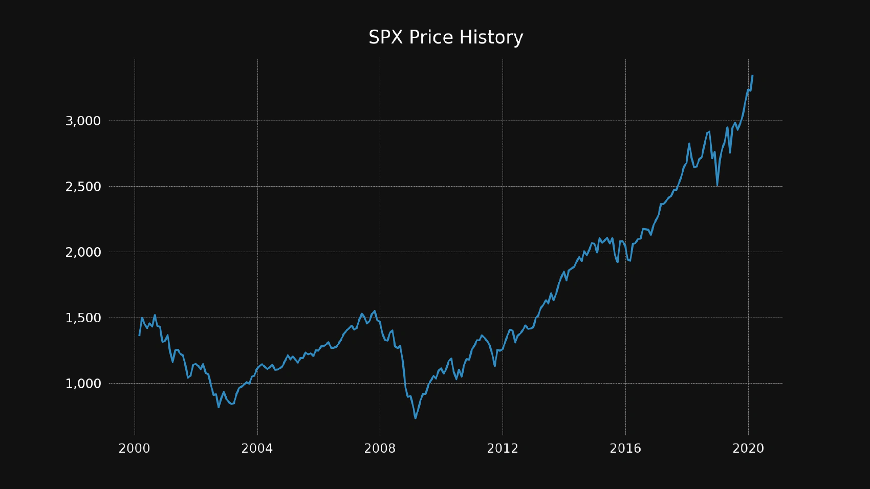
Conclusion
We’ve created a simple wrapper that allows us to query stock price history and used it to plot the data on screen. Next, we’ll use this data to show the risk of different stocks.
Plotting Risk as Variance
Variance is an important indicator if you want to know the level of risk associated with holding a given security. It’s important to understand that past variance might not be a good predictor of future variance, but most of the time it works, and we don’t have other options anyway. Let’s create a script for displaying returns distribution, variance and standard deviation of any given security.
Finding Variance
It’s super easy to find a variance if you have the returns’ data. Here is how to do that:
- Find mean returns (mean of all data points).
- For each data point, subtract its value from the mean returns and square the result of subtraction (note that we made it impossible to have a negative result since no number in the power of 2 can be negative).
- Sum all the results and divide this sum by the number of data points.
That’s all, now you have a variance. If you also want to find a standard deviation, just take the square root of a variance value.
Obtaining The Data
Let’s extend our alpha_vantage.py module to add one more function:
def get_stock_returns_history(symbol: str,
                              interval: Interval) -> [float]:
    price_history = get_stock_price_history(symbol, interval, adjusted=True)

    returns: [float] = []
    prev_price = None

    for item in price_history:
        if prev_price != None:
            returns.append((item.price - prev_price) / prev_price)

        prev_price = item.price

    return returns
This data is based on the price history data, but now we’re not interested in absolute numbers, so we have to calculate relative changes and return them as a simple array. For instance, with a MONTHLY interval this array would contain the month-to-month changes in the price of a given security.
Plotting The Data
Let’s create a new file and call it variance.py, it should contain the following code:
import sys
import numpy as np
import matplotlib
import matplotlib.pyplot as plt
import pathlib
import matplotlib.style as style

import alpha_vantage
from alpha_vantage import Interval
import plot_style


def show_variance(symbol, interval=Interval.MONTHLY):
    returns = alpha_vantage.get_stock_returns_history(symbol, interval)
    variance = np.var(returns)
    standard_deviation = np.sqrt(variance)
    mean_return = np.mean(returns)

    plot_style.hist()

    n, _, patches = plt.hist(returns, density=True, bins=25)

    for item in patches:
        item.set_height(item.get_height() / sum(n))

    max_y = max(n) / sum(n)
    plt.ylim(0, max_y + max_y / 10)

    plt.gca().set_xticklabels(['{:.0f}%'.format(x*100)
                               for x in plt.gca().get_xticks()])

    plt.gca().set_yticklabels(['{:.0f}%'.format(y*100)
                               for y in plt.gca().get_yticks()])

    title_line_1 = f'{symbol.upper()} {interval.value.lower().capitalize()} Return Distribution'
    title_line_2 = 'Standard Deviation = %.2f%% Mean Return = %.2f%%' % (
        standard_deviation * 100, mean_return * 100)
    plt.title(f'{title_line_1}\n{title_line_2}')
    plt.xlabel(f'{interval.value.lower().capitalize()} Return')
    plt.ylabel('Probability')

    pathlib.Path('img/variance').mkdir(parents=True, exist_ok=True)
    plt.savefig(f'img/variance/{symbol}.png')
    plt.close()


show_variance(sys.argv[1])
First, this script checks the number of input parameters, we need this check to find out whether we have a period specified or should we use the default value (MONTHLY). Next, this code fetches the returns’ history data and calculates the variance based on that data. The final step is to plot the returns’ distribution as a histogram, so we can see the relative frequencies of any given returns.
Testing
Let’s test our new module by requiring it to draw a couple of charts:
$ python variance.py tsla
You should see the chart similar to this one:
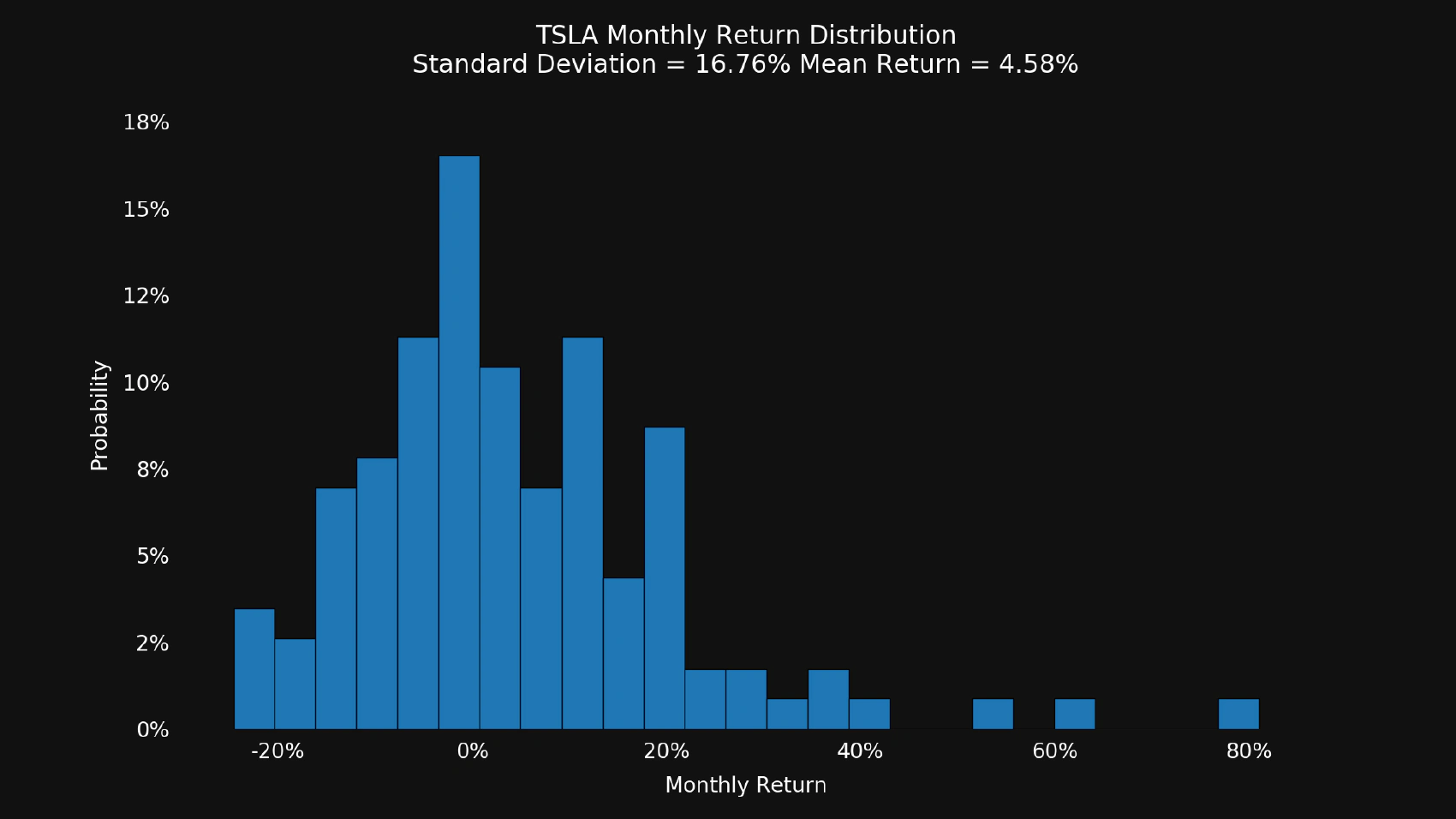
Now let’s check the variance of S&P 500 (SPX) index:
$ python variance.py spx
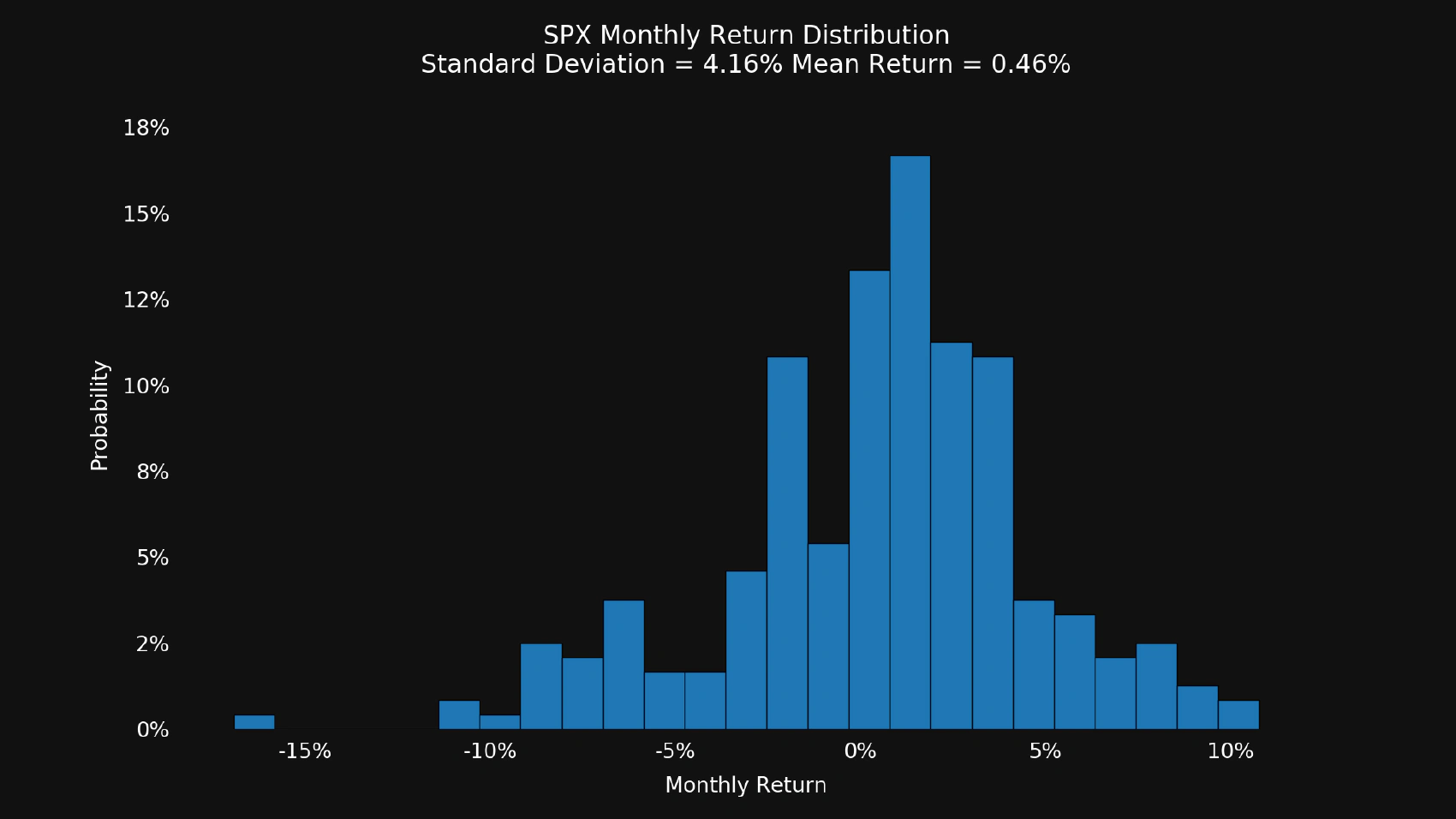
It’s easy to see why TSLA is more risky to hold than SPX but it does not mean that it’s a bad choice. Why does anyone want to hold such an unpredictable stock? You can look at the mean returns or plot the price history to see the answer.
Conclusion
Now that we can get a hint of the risk of holding any particular security, it would be nice to have a way of comparing the returns. It might be a good idea to hold a risky security if it gives exceptional returns, and you are not worried about price volatility in the short term.
Comparing Asset Returns
It’s hard to compare the returns on the given securities just by looking at their price history in absolute terms, so we need to find a better way of comparing historical returns. One of the possible solutions is to adjust the whole data series in such a way that the first data point would be equal to some predefined number. We’re going to adjust the price history of both assets, so they will always start with the same value, let’s say 100. This method allows us to see what would happen with $100 invested in 2 given stocks on the date D.
Data
You should already have a function for retrieving stock price history, if you don’t have it - go to Price History and implement it. It should return all the data we need, but it has 2 major issues:
- The values can have different date ranges, we need to use the same range for both datasets.
- The values are in absolute terms, so we need to adjust them to start with the same value but keep the original proportions.
Adjusting The Range
The most obvious way to solve the range mismatch is to cut out all the dates that are not present in both data sets. Here is the possible solution:
history_1 = alpha_vantage.get_stock_price_history(
    symbol_1, interval, adjusted)

history_2 = alpha_vantage.get_stock_price_history(
    symbol_2, interval, adjusted)

history_1 = [v for v in history_1 if v.date in list(
    i.date for i in history_2)]

history_2 = [v for v in history_2 if v.date in list(
    i.date for i in history_1)]
We just filter each dataset and keep only the dates that are present in the other dataset. Now we can be sure that we’re comparing the same date range.
Adjusting The Values
Different stocks can have different prices at any given time and if some stock is selling for $1000 per share it does not mean that it’s better than the stock trading for $1 per share. It’s all relative, so we have to scale the data before we compare it.
Here’s how we can do that:
def adjust_values(data: List[AssetPrice], start: float):
    scale_factor = None

    for v in data:
        if scale_factor == None:
            scale_factor = v.price / start

        v.price = v.price / scale_factor
Plotting The Data
Let’s create a new file and name it compare.py:
import sys
import pathlib
import matplotlib.pyplot as plt
from typing import List

import alpha_vantage
from alpha_vantage import Interval, AssetPrice
import plot_style


def compare(symbol_1: str,
            symbol_2: str,
            interval=Interval.MONTHLY,
            adjusted=True):
    history_1 = alpha_vantage.get_stock_price_history(
        symbol_1, interval, adjusted)

    history_2 = alpha_vantage.get_stock_price_history(
        symbol_2, interval, adjusted)

    history_1 = [v for v in history_1 if v.date in list(
        i.date for i in history_2)]

    history_2 = [v for v in history_2 if v.date in list(
        i.date for i in history_1)]

    adjust_values(history_1, start=100.0)
    adjust_values(history_2, start=100.0)

    plot_style.line()

    plt.plot(
        list(i.date for i in history_1),
        list(i.price for i in history_1),
        label=symbol_1.upper())

    plt.plot(
        list(i.date for i in history_2),
        list(i.price for i in history_2),
        label=symbol_2.upper())

    title = f'{symbol_1.upper()} vs {symbol_2.upper()}'
    title = title + ' (adjusted)' if adjusted == True else title
    plt.title(title)
    plt.legend()

    pathlib.Path('img/compare').mkdir(parents=True, exist_ok=True)
    plt.savefig(f'img/compare/{symbol_1.lower()}-{symbol_2.lower()}.png')
    plt.close()


def adjust_values(data: List[AssetPrice], start: float):
    scale_factor = None

    for v in data:
        if scale_factor == None:
            scale_factor = v.price / start

        v.price = v.price / scale_factor


compare(sys.argv[1], sys.argv[2])
This code combines the previous steps and also draws the resulting datasets on the screen.
Testing
Let’s test this module by comparing the Tesla Inc cumulative returns using the S&P 500 index as a benchmark:
python compare.py spx tsla
You should see the chart similar to this one:
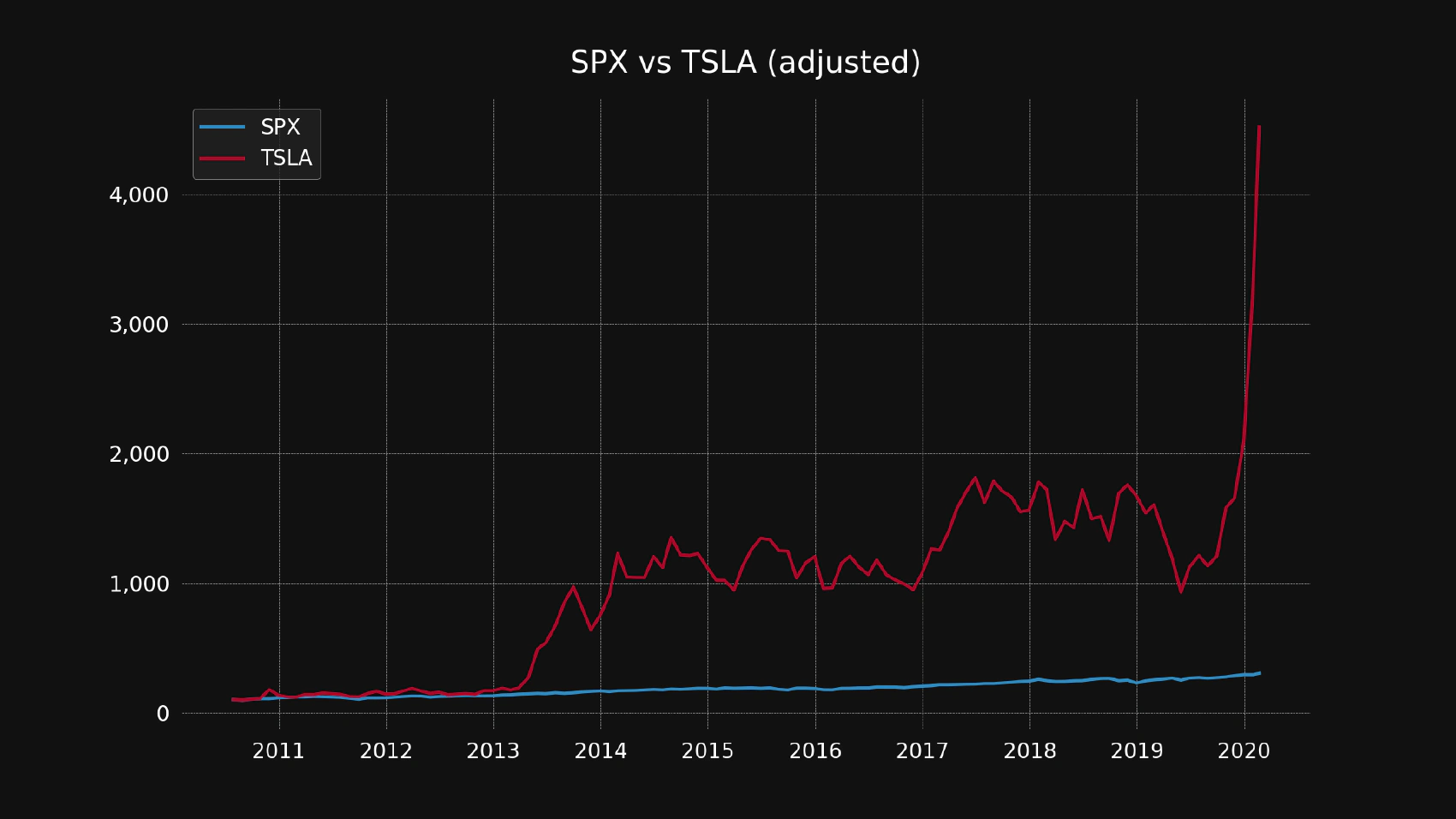
It seems like the TSLA stock made much more money for its shareholders than the SPX index, but it also looks more volatile and jittery.
Conclusion
Now we have a tool for comparing asset performance, and it also gives us a hint about the historical volatility. Next, we’ll create a tool for measuring the “compatibility” of 2 given stocks. Expected returns might be a good hint on what to buy, but it’s also important to understand the relationship between different stocks in a portfolio.
Plotting Efficient Frontier (2 assets)
The main idea behind the Efficient Frontier is that the overall risk (volatility) of a portfolio may not be equal to the sum of the risk of its components, so some combinations are better than others. In this post we’re going to visualize the optimal weights of 2 given assets in a hypothetical portfolio.
Components
Let’s compare IBM and Disney (DIS):
python compare.py ibm dis
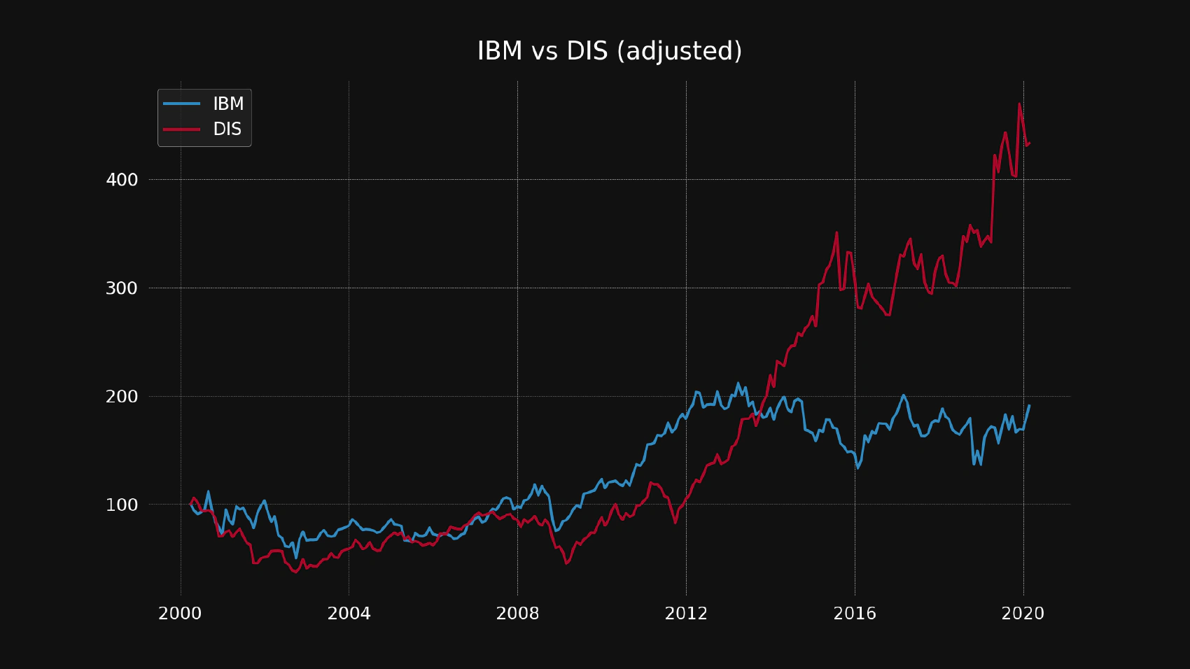
It looks like both of those stocks have made a lot of money for their shareholders, but it’s unclear who will be better off in the long run. Let’s analyze both stocks in order to make a few assumptions based on their historical performance.
Stats
Here are some stats for IBM:
- Monthly mean return: 0.76%
- Standard deviation of monthly return: 7.51%
Here are the same stats tor DIS:
- Monthly mean return: 0.83%
- Standard deviation of monthly return: 7.25%
Those stocks look pretty close in terms of risk and return so which one should we choose? Would it be a better idea to split the portfolio 50/50? Let’s run a few calculations to find out.
Diversified Portfolio
So what are the mean return of the 50/50 portfolio? It’s just a weighted average of its components’ return:
$$ r_p = r_1 w_1 + r_2 w_2 $$
Where:
\( r_p \) = portfolio mean return
\( r_1, r_2 \) = return of the portfolio components
\( w_1, w_2 \) = weights of the portfolio components
0.76% * 50% + 0.83% * 50% = 0.80%
Not bad, but what about the risk? Here is the formula:
$$ σ_p^2 = w_1^2 σ_1^2 + w_2^2 σ_2^2 + 2 w_1 w_2 cov(1, 2) $$
In our case, covariance is 0.00207, so:
- variance = 0.5^2 * 0.0751^2 + 0.5^2 * 0.0725^2 + 2 * 0.5 * 0.5 * 0.00207 = 0.003759065
- standard deviation = 6.13% (square root of variance)
It looks like the 50/50 split is not a bad idea after all, we would get the same return with significantly less risk but what about the other possible combinations? How much would we get if we were ready to accept more risk? Is it possible to decrease the risk? Plotting many combinations on a graph might give us a good picture of how diversification works and helps us to make the right choice.
Plotting Portfolios
Let’s plot a lot of different asset combinations in order to find out how they affect portfolio volatility and expected return. A scatter plot is a good tool for showing that kind of data. Here is the script, you can call it frontier2.py:
import sys
import pathlib
import numpy as np
import matplotlib
import matplotlib.pyplot as plt

import alpha_vantage
from alpha_vantage import Interval
import plot_style


def show_frontier(symbol1: str,
                  symbol2: str,
                  interval=Interval.MONTHLY):
    returns1 = alpha_vantage.get_stock_returns_history(symbol1, interval)
    returns2 = alpha_vantage.get_stock_returns_history(symbol2, interval)

    if len(returns1) > len(returns2):
        returns1 = returns1[-len(returns2):]

    if len(returns2) > len(returns1):
        returns2 = returns2[-len(returns1):]

    mean_returns1 = np.mean(returns1)
    variance1 = np.var(returns1)
    standard_deviation1 = np.sqrt(variance1)

    #print(f'Mean returns ({symbol1}) = {mean_returns1}')
    #print(f'Variance ({symbol1}) = {variance1}')
    #print(f'Standard Deviation ({symbol1}) = {standard_deviation1}')

    mean_returns2 = np.mean(returns2)
    variance2 = np.var(returns2)
    standard_deviation2 = np.sqrt(variance2)

    #print(f'Mean returns ({symbol2}) = {mean_returns2}')
    #print(f'Variance ({symbol2}) = {variance2}')
    #print(f'Standard Deviation ({symbol2}) = {standard_deviation2}')

    correlation = np.corrcoef(returns1, returns2)[0][1]
    #print(f'Corellation = {correlation}')

    weights = []

    for n in range(0, 101):
        weights.append((1 - 0.01 * n, 0 + 0.01 * n))

    returns = []
    standard_deviations = []

    portfolio_50_50_standard_deviation = None
    portfolio_50_50_returns = None

    plot_style.scatter()

    for w1, w2 in weights:
        returns.append(w1 * mean_returns1 + w2 * mean_returns2)

        variance = w1**2 * standard_deviation1**2 + w2**2 * standard_deviation2**2 + \
            2 * w1 * w2 * standard_deviation1 * standard_deviation2 * correlation

        standard_deviation = np.sqrt(variance)
        standard_deviations.append(standard_deviation)

        plt.scatter(standard_deviations[-1], returns[-1], color='#007bff')

        if w1 == 0.5 and w2 == 0.5:
            portfolio_50_50_standard_deviation = standard_deviations[-1]
            portfolio_50_50_returns = returns[-1]

    plt.scatter(portfolio_50_50_standard_deviation,
                portfolio_50_50_returns, marker='x', color='red', alpha=1, s=320)

    x_padding = np.average(standard_deviations) / 25

    plt.xlim(min(standard_deviations) - x_padding,
             max(standard_deviations) + x_padding)

    y_padding = np.average(returns) / 25

    plt.ylim(min(returns) - y_padding, max(returns) + y_padding)

    plt.gca().set_xticklabels(['{:.2f}%'.format(x*100)
                               for x in plt.gca().get_xticks()])
    plt.gca().set_yticklabels(['{:.2f}%'.format(y*100)
                               for y in plt.gca().get_yticks()])

    plt.title(f'Efficient Frontier ({symbol1.upper()} and {symbol2.upper()})')

    plt.xlabel(f'Risk ({interval.value.lower().capitalize()})')
    plt.ylabel(f'Return ({interval.value.lower().capitalize()})')

    pathlib.Path('img/frontier2').mkdir(parents=True, exist_ok=True)
    plt.savefig(f'img/frontier2/{symbol1.lower()}-{symbol2.lower()}.png')
    plt.close()


show_frontier(sys.argv[1], sys.argv[2])
Now let’s run this script in order to see the scatter plot:
python frontier2.py ibm dis
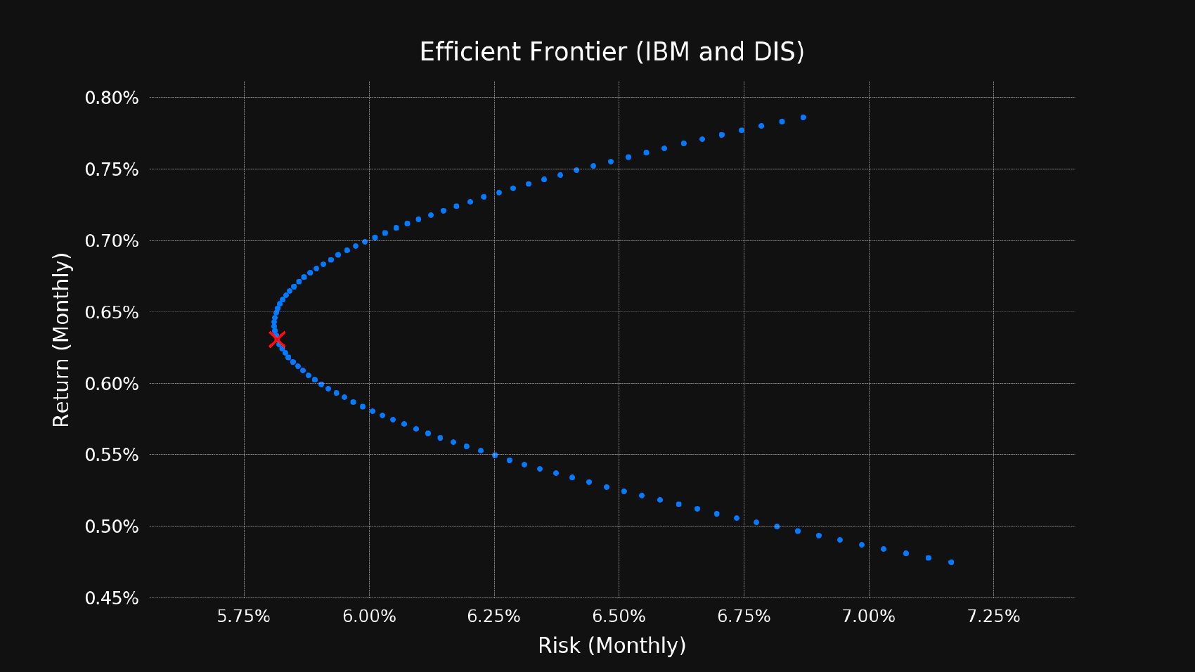
As you can see, the 50/50 portfolio is on the bottom half of this chart. That’s not very good because it means that there is another portfolio that has more returns with the same risks. Usually, it’s better to ignore the bottom half of the efficient frontier and pick a portfolio from the top half that best suits your risk tolerance. Many young people prefer high returns, and it might be a good idea if your investment horizon is long enough, but the people who are close to retirement age are typically not comfortable with the idea of waiting for another 20-30 years in order to recover from a possible loss caused by holding too many high-risk assets.
Conclusion
Now we have a script that allows us to find an optimal combination of 2 different assets. That’s a good start, but it’s more practical to be able to include more assets and that’s what we’re going to do next.
Plotting Efficient Frontier (N assets)
We already have the efficient frontier script, but it has one major limitation: it does not allow us to plot more than two assets. Plotting two assets is enough to see diversification in action, but it’s not practical to have a portfolio that consists of two assets. In this post we’re going to extend the previous script in order to support an arbitrary number of assets.
Why Diversify?
Diversification helps to reduce portfolio volatility but to what extent? Well, it depends on the correlations between different assets, but we can safely assume that the number of assets should be greater than 2. If you decide to add another asset, the smaller the number of assets you already have in your portfolio, the better the effect of diversification. Here is the picture that helps to visualize how the number of assets affects the portfolio risk:
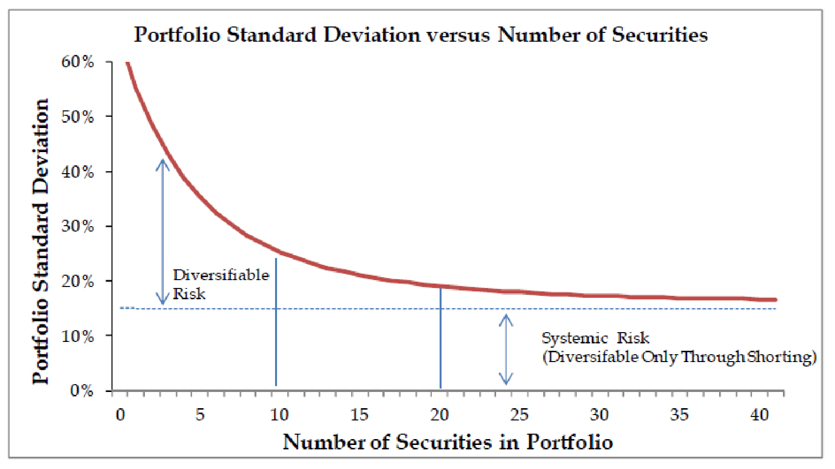
As you can see, one thing is clear: having two assets does not allow us to get all the benefits of diversification. There are many opinions on what number of assets is “right” but almost everyone agrees that two is far too low.
Goal
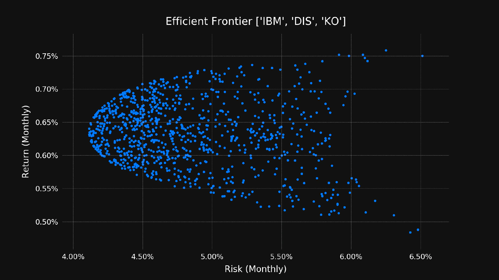
We already calculated the efficient frontier for a portfolio that consists of the IBM and DIS stocks. Let’s add one more stock to it. You can pick any stock or an index, but I’ll go with Coca-Cola (KO).
So, how do we calculate our risks and rewards?
Expected Return
Here is how we can calculate the expected return on a portfolio:
$$ E(R_p) = \sum_{i=1}^N w_i E(R_i) $$
Where:
\( r_p \) = expected return on a portfolio
\( N \) = number of assets in a portfolio
\( w_i \) = weight of an asset i in a portfolio
\( R_i \) = expected return on asset i
All of this is pretty simple, we just need to find the weighted average of the returns of every asset in a portfolio.
Variance
Variance is a bit more tricky to calculate because we have to include the correlations between each pair of assets:
$$ σ_p^2 = \sum_{i=1}^N w_i^2 σ_i^2 + \sum_{i=1}^N \sum_{j \not = i}^N w_i w_j σ_i σ_j p_{ij} $$
Where:
\( σ_p^2 \) = portfolio volatility
\( w_i \) = weight of an asset i in a portfolio
\( σ_i \) = standard deviation of an asset i
\( p_{ij} \) = correlation of returns between the assets i and j
Standard Deviation
Standard deviation of a portfolio is just a square root of its variance:
$$ σ_p = (σ_p^2)^{1 \over 2} $$
That gives us a hint about the portfolio riskiness.
Implementation
Let’s create a new file and call it frontier.py:
import matplotlib.pyplot as plt
import sys
import pathlib
import numpy as np

import alpha_vantage
from alpha_vantage import Interval
import plot_style


def show_frontier(symbols, interval=Interval.MONTHLY):
    #print(f'Symbols: {symbols}')

    returns_history = dict()

    min_length = None

    for symbol in symbols:
        history = alpha_vantage.get_stock_returns_history(symbol, interval)
        #print(f'Fetched {len(history)} records for symbol {symbol}')

        if min_length == None:
            min_length = len(history)

        if (len(history) < min_length):
            min_length = len(history)

        returns_history[symbol] = history

    #print(f'Min hisotry length = {min_length}')

    for symbol in symbols:
        returns_history[symbol] = returns_history[symbol][-min_length:]

    # for symbol in symbols:
    #    print(
    #       f'History for symbol {symbol} has {len(returns_history[symbol])} records')

    mean_returns = dict()
    variances = dict()
    standard_deviations = dict()

    for symbol in symbols:
        history = returns_history[symbol]
        history_length = len(history)
        #print(f'Return history for symbol {symbol} has {history_length} records')
        mean_returns[symbol] = np.mean(history)
        variances[symbol] = np.var(history)
        standard_deviations[symbol] = np.sqrt(variances[symbol])

    plot_style.scatter()

    portfolio_returns = []
    portfolio_deviations = []

    for i in range(0, 1_000):
        randoms = np.random.random_sample((len(symbols),))
        weights = [random / sum(randoms) for random in randoms]

        expected_return = sum([weights[i] * mean_returns[symbol]
                               for i, symbol in enumerate(symbols)])

        weights_times_deviations = [
            weights[i]**2 * standard_deviations[s]**2 for i, s in enumerate(symbols)]
        variance = sum(weights_times_deviations)

        for i in range(0, len(symbols)):
            for j in range(0, len(symbols)):
                if (i != j):
                    symbol1 = symbols[i]
                    symbol2 = symbols[j]
                    #print('Pair = %s %s' % (symbol1, symbol2))

                    weight1 = weights[i]
                    weight2 = weights[j]
                    #print('Weights = %s %s' % (weight1, weight2))

                    deviation1 = standard_deviations[symbol1]
                    deviation2 = standard_deviations[symbol2]
                    #print('Deviations = %s %s' % (deviation1, deviation2))

                    correlation = np.corrcoef(
                        returns_history[symbol1], returns_history[symbol2])[0][1]
                    #print('Correlation = %f' % correlation)

                    additional_variance = weight1 * weight2  \
                        * deviation1 * deviation2 \
                        * correlation
                    #print('Additional variance = %f' % additional_variance)

                    variance += additional_variance

        standard_deviation = np.sqrt(variance)
        #print('Portfolio expected return = %f' % expected_return)
        #print('Portfolio standard deviation = %f' % standard_deviation)

        plt.scatter(standard_deviation, expected_return, color='#007bff')

        portfolio_returns.append(expected_return)
        portfolio_deviations.append(standard_deviation)

    x_padding = np.average(portfolio_deviations) / 25
    plt.xlim(min(portfolio_deviations) - x_padding,
             max(portfolio_deviations) + x_padding)

    y_padding = np.average(portfolio_returns) / 25
    plt.ylim(min(portfolio_returns) - y_padding,
             max(portfolio_returns) + y_padding)

    plt.gca().set_xticklabels(['{:.2f}%'.format(x*100)
                               for x in plt.gca().get_xticks()])
    plt.gca().set_yticklabels(['{:.2f}%'.format(y*100)
                               for y in plt.gca().get_yticks()])

    plt.title(f'Efficient Frontier {list(s.upper() for s in symbols)}')

    plt.xlabel(f'Risk ({interval.value.lower().capitalize()})')
    plt.ylabel(f'Return ({interval.value.lower().capitalize()})')

    pathlib.Path('img/frontier').mkdir(parents=True, exist_ok=True)
    plt.savefig(f'img/frontier/frontier.png')
    plt.close()


show_frontier(sys.argv[1:])
Testing
Now, let’s run our new script in order to see the efficient frontier:
python frontier.py ibm dis ko
You should see the following image:
Conclusion
Now we are able to plot the efficient frontier based on an arbitrary number of assets. Please note that nothing is “for sure” in the world of investing and this model has a lot of limitations, although it’s probably one of the best models that are currently available. Our expected return is based purely on the past performance which might not be an accurate assumption about the future.
Another thing to consider is the limit of diversification. The benefits of having more assets tend to wear off with each new asset added to your portfolio. There is a huge difference between the 2-asset and 10-asset portfolios but there might be no gain in having 200 assets, especially if you take into account all the transaction costs of re-balancing your portfolio.